
June 06, 2017
The workspace for our haptic interface arm was really small, so it was hard to tell what the arm was drawing when moving autonomously, or for the user to tell what was going on when he/she was moving around the effector. I had D3 plot the position of the effector as it was moving around, so we could clearly demonstrate the precision with which our control system was drawing. It also came in handy for testing out our math, and testing in general, to make sure we were actually drawing shapes and performing desired movement, and not just watching/feeling the effector move around doing diddly squat.
Here’s an old video of us testing out the real time plotting (I know it’s dark, but look at the top right to see the arm moving around):
Here is an early screenshot of the something the arm drew that the D3 plot captured:
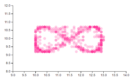
Ignore the scale - I had a scaling factor making it proportionally too large in either direction in the math at first. As you can see, the density of dots reflects the most frequent positions of the effector. You’ll notice some faint pink dots - early on, the effector had a bit of shake to it. The faint pink dots which strayed from the desired path indicated that we needed to tune our system more.
Here is a screenshot of a more finely tuned design:
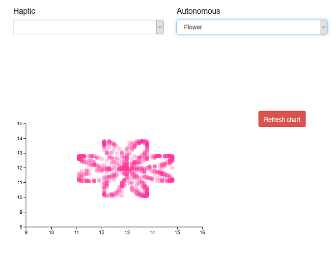
I guess the sin function we used could have used a vertical scaling factor a tad bit larger, but notice that the system in this plot had much steadier control.
We had the dots drawn in dark blue as the effector reached each position, then used an animation to fade them purple, then to pink. These screenshots were taken after the whole animation had faded to pink.
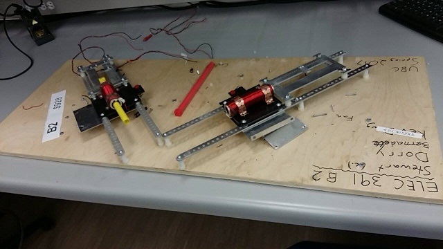
I couldn’t find much on real time data visualizations in D3. For the most part, I could only find demos which updated D3 graphs say, every 1-5 seconds. This wasn’t good enough for what we needed. We needed a plot that could instantaneously reflect minute changes of the effector position in our workspace. Unfortunately I am writing this post over 2 months after completing the project, but our workspace was only a few cm long and a few cm wide (maybe 4cm? The scale is wrong in some of the screenshots I took, as early on I had entered the arm length of the robot arm wrong and it increased the scale of everything by a factor…took us like two hours to figure out what was going wrong, har har…). Precision and changes in movement were detected for +/- 0.001cm, if I remember correctly…it may have been even more precise than that. I wish I could just run the thing again and check, but after we demoed the project we ripped it apart to salvage parts. So our project now looks like this:
I may write a tutorial on it later, but this post will summarize what I did to create a D3 plot which plotted movement of the robot arm effector, plotting what it drew on a web application. Along with D3.js I used, Node.js and ExpressJS, the serialPort library on npm, and Socket.io.
Here’s what the setup of our project looked like:

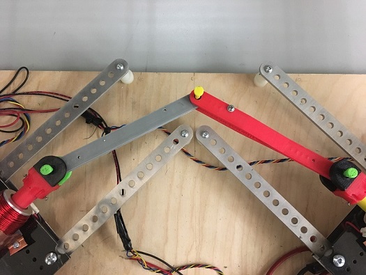
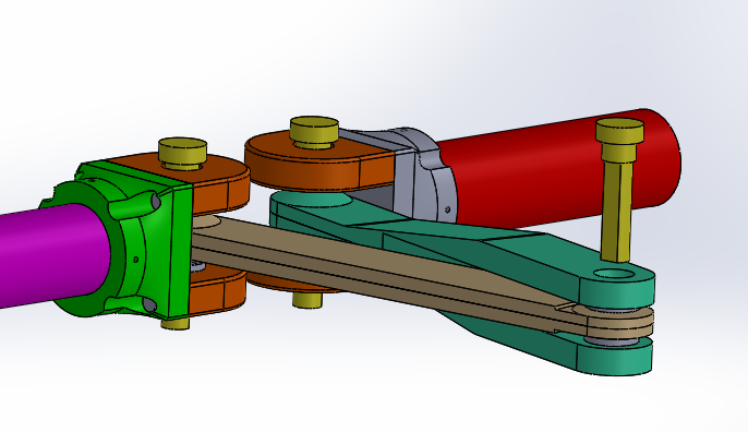
Our project was essentially two linear motors attached to an arm with a joint. As the rotor of the linear motors were moved back and forth, the position of the joint (the effector - the yellow dot in the picture below) would move. We attached a slide potentiometer to each of the linear motors to measure how far in and out they had moved at each given moment based on their readings.
Angled view of arm assembly in AutoCad:
This is a summary of what I did to set up communication with the D3 plot, if you don’t want to read the whole post:
Used Node.js to serve the application off of, used ExpressJS as middleware
Used Socket.io to communicate between the web client and server
Used the serialport library to connect Node.js to my computer’s serial port. Using this library you could write directly to the serial port by writing to the Node.js server (ie through a console.log()), and directly to the Node.js server by writing to the serial port. This latter in my case would be doing Serial.println()’s from the Arduino, for example (Serial.println() was actually too slow for our purposes, but I’ll write more on how we worked around that later).
Used Socket.io to establish communication between the web client and server. We would have the microcontroller take in readings from the two potentiometers, then send the readings to the Node.js server, which would send it to the client through the web socket. At first I had the client do all of our math with the reading values to calculate effector position, as we weren’t that confident in our solution. This way we could move the effector to different positions and view the output on the D3 graph to make sure the output of our calculations was effectively matching our movements
Used D3.js after parsing the string readings to render calculated position value on scatter plot, based on the two potentiometer readings at a given moment. Added in animations for prettiness.
First, we needed a way to communicate between hardware and software. That is, we needed the microcontroller to send information on the effector position to the Node.js server.
There wasn’t tons out there that really supported our needs - Johnny Five has become pretty popular library for using JS to conrol Arduino, Raspberry Pi, and various other hobby microcontrollers. It’s moreso a solution to replace doing your firmware in JS instead of C, however. This wouldn’t work as the rest of my team was familiar with C, and additionally we did not want to slow down our system by using JS. Our control system was extremely time sensitive - it may have been a risk, adding on the compile time of JS. On top of this Johnny Five works by creating objects for different components in your circuit, and then calling functions for those objects. This would limit us to whatever objects the Johnny Five library supported. Sure they have buttons, LED’s and basic sensors, but sometimes we needed very specific components, and didn’t want to run into the problem of them not being supported. For example, the slide potentiometers we were using were exponential, and I don’t think Johnny Five would just happen to have an exponential potentiometer built into the library which perfectly matched the exponential curve and calibration at which ours increased at.
Another problem is that we needed constant bidirectional communication between the hardware and software, and Johnny Five is designed for one way - it is mostly for writing commands to the hardware, and not the other way around.
I chose the serialPort library because we could keep coding for our microcontroller in C, and communicate with the web server by simply writing to the serial port. From the server we could send the received strings from the microcontroller to the client through a web socket.
We sent over the potentiometer readings between start and stop characters so we could define each individual reading and which potentiometer it belonged to. Readings from the left potentiometer were sent as, for example, B1020E, and readings from the right potentiometer were sent as C108E.
After parsing the left and right readings on the client side and then displaying the respective calculated x and y positions on the D3 plot, we could move the effector around and try to draw shapes, and ensure the software was accurately reflecting movement. This was part of our testing process to make sure our math was working. Eventually, we applied math with the potentiometer readings all on the microcontroller in C, then sent the calculatex x and y positions between the start and stop characters.
It got really difficult not messing up the timing of our control system with Serial.println(). These constant prints got expensive, and would mess up the control system and cause the arm to go out of control. This was probably related to the fact that we were using a measly Arduino Uno, which has pretty limited clock speed… not that Arduino Uno isn’t amazing, but near the end of the project we realized how the extra clock speed of an Arduino Mega or some fancier microcontroller would have helped a lot. We couldn’t send our data through interrupts either, as Serial.println()’s in the Arduino Uno interfere with the ISR. I ended up having to write a custom parser with sprintf() (much less expensive) to send over our data through the microcontroller, instead of just using normal prints:
	void write_to_serial(float x, float y){
	      char xStr[6];
	      if( x < 10){
	        char xBuffer[1];
	        dtostrf(x,2,3,xBuffer);
	        sprintf(xStr, "%c%c%c%c%c", beginR, xBuffer[0],xBuffer[1],xBuffer[2],endR);
	      }
	      else{
	        char xBuffer[2];
	        dtostrf(x,2,3,xBuffer);
	        sprintf(xStr, "%c%c%c%c%c%c", beginR, xBuffer[0],xBuffer[1],xBuffer[2],xBuffer[3],endR);
	      }
	      Serial.write(xStr);

	      char yStr[6];
	      if( y < 10){
	        char yBuffer[1];
	        dtostrf(y,2,3,yBuffer);
	        sprintf(yStr, "%c%c%c%c%c", beginL, yBuffer[0],yBuffer[1],yBuffer[2],endL);
	      }
	      else{
	        char yBuffer[2];
	        dtostrf(y,2,3,yBuffer);
	        sprintf(yStr, "%c%c%c%c%c%c", beginL, yBuffer[0],yBuffer[1],yBuffer[2],yBuffer[3],endL);
	      }
	      Serial.write(yStr);
	}
Initially I struggled a lot with getting the client to consistently communicate with the microcontroller. Sometimes it just did nothing and failed silently, and wasn’t receiving or updating the incoming string data. One of the biggest game changers was discovering the parser property when setting up the serialPort on the server. With this property in serialPort library, you can set the end character and have serialPort automatically split your string when it sees it in incoming data. This ENORMOUSLY improved performance. Here are the settings I instantiated serialPort with:
	var port = new SerialPort("COM6", {   //*change this to COM port arduino is on
	       baudrate: 9600,
	       parser: SerialPort.parsers.readline("E"),
	       dataBits: 8,
	       parity: 'none',
	       stopBits: 1,
	       flowControl: false
	  });
And this is the client side parsing we then used:
	socket.on('updatePot', function(data){
	    unParsedData += data;
	    if(unParsedData.charAt(0) === "B"){
	        console.log("in if x:" + unParsedData);
	        rightReading = unParsedData.substring(unParsedData.indexOf('B')+1);
	        console.log("x: " + rightReading);
	        dataset.push([rightReading,leftReading]);
	        unParsedData = ""; //reset string that receives data
	        update(); //update d3 scatterplot
	    }
	    //left potentiometer reading
	    if(unParsedData.charAt(0) === "C"){
	        console.log("in if y:" + unParsedData);
	        leftReading = unParsedData.substring(unParsedData.indexOf('C')+1);
	        console.log("y: " + leftReading);
	        unParsedData = "";
	        dataset.push([rightReading,leftReading]);
	        update(); //update d3 scatterplot
	    }
});I’m hoping I can skip the details and basics of D3 here. Basically, I created the initial scatter plot like this:
	var xAxis = d3.svg.axis()
	    .scale(xScale)
	    .orient("bottom")
	    .ticks(10);

	// Define Y axis
	var yAxis = d3.svg.axis()
	    .scale(yScale)
	    .orient("left")
	    .ticks(10);

	// Create SVG element
	var svg = d3.select("#scatter-plot")  // This is where we put our vis
	    .append("svg")
	    .attr("width", canvas_width)
	    .attr("height", canvas_height)

	// Create Circles
	svg.selectAll("circle")
	    .data(dataset)
	    .enter()
	    .append("circle")  // Add circle svg
	    .attr("cx", function(d) {
	        return xScale(d[0]);  // Circle's X
	    })
	    .attr("cy", function(d) {  // Circle's Y
	        return yScale(d[1]);
	    })
	    .attr("r", 2)
	    .on("mouseover", function(d) {
	            tooltip.transition()
	                .duration(50)
	                .style("opacity", .9);
	            div .html(xScale(d[0]) + "<br/>"  + yScale(d[1]))
	                .style("left", (d3.event.pageX) + "px")
	                .style("top", (d3.event.pageY - 28) + "px");
	            })
	        .on("mouseout", function(d) {
	            tooltip.transition()
	                .duration(50)
	                .style("opacity", 0);
	        });  // radius
The plot would intially start out empty. If you look back up at the client parsing code, you’ll notice it is wrapped in a socket event, which is triggered when new incoming data comes in from the server/microcontroller. Once the new data is parsed, it is pushed to a local array (either the array for the right or left motor’s position), and the update() function is called, which plots the new x,y coordinates on the scatter plot:
	function update() {
	    // Update scale domains
	    xScale.domain([xmin, xmax]);

	    yScale.domain([ymin,ymax]);

	    //render newly added elements of array
	    var dataSelection = svg.selectAll("circle")
	                            .data(dataset);

	    dataSelection.enter()
	        .append("circle")  // Add circle svg
	        .attr("cx", function(d) {
	            return xScale(d[0]);  // Circle's X
	        })
	        .attr("cy", function(d) {  // Circle's Y
	            return yScale(d[1]);
	        })
	        .attr("fill", "blue")
	        .attr("r", 6.5);

	  // Update circles
	    svg.selectAll("circle")
	        .data(dataset)  // Update with new data
	        .transition()  // Transition from old to new
	        .attr("cx", function(d) {
	            return xScale(d[0]);  // Circle's X
	        })
	        .attr("cy", function(d) {
	            return yScale(d[1]);  // Circle's Y
	        })
	        .each("end", function() {  // End animation
	            d3.select(this)  // 'this' means the current element
	            .transition()
	            .duration(500)
	            .attr("fill", "#ff3399")  // Change color
	            .attr("r", 5);  // Change radius
	        });

	    // Update X Axis
	    svg.select(".x.axis")
	        .transition()
	        .duration(1000)
	        .call(xAxis);

	    // Update Y Axis
	    svg.select(".y.axis")
	       .transition()
	       .duration(100)
	       .call(yAxis);
	}